Fast wavelet transform
Algorithm
The fast wavelet transform is a mathematical algorithm designed to turn a waveform or signal in the time domain into a sequence of coefficients based on an orthogonal basis of small finite waves, or wavelets. The transform can be easily extended to multidimensional signals, such as images, where the time domain is replaced with the space domain. This algorithm was introduced in 1989 by Stéphane Mallat.[1]
It has as theoretical foundation the device of a finitely generated, orthogonal multiresolution analysis (MRA). In the terms given there, one selects a sampling scale J with sampling rate of 2J per unit interval, and projects the given signal f onto the space ; in theory by computing the scalar products


where is the scaling function of the chosen wavelet transform; in practice by any suitable sampling procedure under the condition that the signal is highly oversampled, so

:=\sum _{n\in \mathbb {Z} }s_{n}^{(J)}\,\varphi (2^{J}x-n)}](https://wikimedia.org/api/rest_v1/media/math/render/svg/9b024490cfc2a80bfcae14105c5ad5c52c87c750)
is the orthogonal projection or at least some good approximation of the original signal in .
The MRA is characterised by its scaling sequence
- or, as Z-transform,


and its wavelet sequence
- or


(some coefficients might be zero). Those allow to compute the wavelet coefficients , at least some range k=M,...,J-1, without having to approximate the integrals in the corresponding scalar products. Instead, one can directly, with the help of convolution and decimation operators, compute those coefficients from the first approximation .


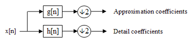
Forward DWT
For the discrete wavelet transform (DWT), one computes recursively, starting with the coefficient sequence and counting down from k = J - 1 to some M < J,
- or


and
- or ,


for k=J-1,J-2,...,M and all . In the Z-transform notation:


- The downsampling operator reduces an infinite sequence, given by its Z-transform, which is simply a Laurent series, to the sequence of the coefficients with even indices, .
- The starred Laurent-polynomial denotes the adjoint filter, it has time-reversed adjoint coefficients, . (The adjoint of a real number being the number itself, of a complex number its conjugate, of a real matrix the transposed matrix, of a complex matrix its hermitian adjoint).
- Multiplication is polynomial multiplication, which is equivalent to the convolution of the coefficient sequences.


It follows that
:=\sum _{n\in \mathbb {Z} }s_{n}^{(k)}\,\varphi (2^{k}x-n)}](https://wikimedia.org/api/rest_v1/media/math/render/svg/4625f2eab78f08529b341836286918c60e60f868)
is the orthogonal projection of the original signal f or at least of the first approximation onto the subspace , that is, with sampling rate of 2k per unit interval. The difference to the first approximation is given by
}](https://wikimedia.org/api/rest_v1/media/math/render/svg/f932869ac2fffdfa305dde6eea75a24b394fa3af)

=P_{k}[f](x)+D_{k}[f](x)+\dots +D_{J-1}[f](x),}](https://wikimedia.org/api/rest_v1/media/math/render/svg/ad6766a74ca82db487d2d09f0e7a3c6186e296b8)
where the difference or detail signals are computed from the detail coefficients as
:=\sum _{n\in \mathbb {Z} }d_{n}^{(k)}\,\psi (2^{k}x-n),}](https://wikimedia.org/api/rest_v1/media/math/render/svg/4451a9753019f068e1efa436ffc905d20ac0bd1a)
with denoting the mother wavelet of the wavelet transform.

Inverse DWT
Given the coefficient sequence for some M < J and all the difference sequences , k = M,...,J − 1, one computes recursively


- or


for k = J − 1,J − 2,...,M and all . In the Z-transform notation:
- The upsampling operator creates zero-filled holes inside a given sequence. That is, every second element of the resulting sequence is an element of the given sequence, every other second element is zero or . This linear operator is, in the Hilbert space , the adjoint to the downsampling operator .


See also
References
- S.G. Mallat "A Theory for Multiresolution Signal Decomposition: The Wavelet Representation" IEEE Transactions on Pattern Analysis and Machine Intelligence, vol. 2, no. 7. July 1989.
- I. Daubechies, Ten Lectures on Wavelets. SIAM, 1992.
- A.N. Akansu Multiplierless Suboptimal PR-QMF Design Proc. SPIE 1818, Visual Communications and Image Processing, p. 723, November, 1992
- A.N. Akansu Multiplierless 2-band Perfect Reconstruction Quadrature Mirror Filter (PR-QMF) Banks US Patent 5,420,891, 1995
- A.N. Akansu Multiplierless PR Quadrature Mirror Filters for Subband Image Coding IEEE Trans. Image Processing, p. 1359, September 1996
- M.J. Mohlenkamp, M.C. Pereyra Wavelets, Their Friends, and What They Can Do for You (2008 EMS) p. 38
- B.B. Hubbard The World According to Wavelets: The Story of a Mathematical Technique in the Making (1998 Peters) p. 184
- S.G. Mallat A Wavelet Tour of Signal Processing (1999 Academic Press) p. 255
- A. Teolis Computational Signal Processing with Wavelets (1998 Birkhäuser) p. 116
- Y. Nievergelt Wavelets Made Easy (1999 Springer) p. 95
Further reading
G. Beylkin, R. Coifman, V. Rokhlin, "Fast wavelet transforms and numerical algorithms" Comm. Pure Appl. Math., 44 (1991) pp. 141–183 doi:10.1002/cpa.3160440202 (This article has been cited over 2400 times.)


