Karger's algorithm

In computer science and graph theory, Karger's algorithm is a randomized algorithm to compute a minimum cut of a connected graph. It was invented by David Karger and first published in 1993.^[1]

The idea of the algorithm is based on the concept of contraction of an edge ${\displaystyle (u,v)}$ in an undirected graph ${\displaystyle G=(V,E)}$. Informally speaking, the contraction of an edge merges the nodes ${\displaystyle u}$ and ${\displaystyle v}$ into one, reducing the total number of nodes of the graph by one. All other edges connecting either ${\displaystyle u}$ or ${\displaystyle v}$ are "reattached" to the merged node, effectively producing a multigraph. Karger's basic algorithm iteratively contracts randomly chosen edges until only two nodes remain; those nodes represent a cut in the original graph. By iterating this basic algorithm a sufficient number of times, a minimum cut can be found with high probability.

The global minimum cut problem

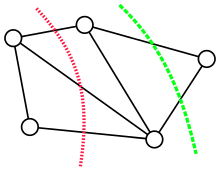
A cut ${\displaystyle (S,T)}$ in an undirected graph ${\displaystyle G=(V,E)}$ is a partition of the vertices ${\displaystyle V}$ into two non-empty, disjoint sets ${\displaystyle S\cup T=V}$. The cutset of a cut consists of the edges ${\displaystyle \{\,uv\in E\colon u\in S,v\in T\,\}}$ between the two parts. The size (or weight) of a cut in an unweighted graph is the cardinality of the cutset, i.e., the number of edges between the two parts,

${\displaystyle w(S,T)=|\{\,uv\in E\colon u\in S,v\in T\,\}|\,.}$

There are ${\displaystyle 2^{|V|}}$ ways of choosing for each vertex whether it belongs to ${\displaystyle S}$ or to ${\displaystyle T}$, but two of these choices make ${\displaystyle S}$ or ${\displaystyle T}$ empty and do not give rise to cuts. Among the remaining choices, swapping the roles of ${\displaystyle S}$ and ${\displaystyle T}$ does not change the cut, so each cut is counted twice; therefore, there are ${\displaystyle 2^{|V|-1}-1}$ distinct cuts. The minimum cut problem is to find a cut of smallest size among these cuts.

For weighted graphs with positive edge weights ${\displaystyle w\colon E\rightarrow \mathbf {R} ^{+}}$ the weight of the cut is the sum of the weights of edges between vertices in each part

${\displaystyle w(S,T)=\sum _{uv\in E\colon u\in S,v\in T}w(uv)\,,}$

which agrees with the unweighted definition for ${\displaystyle w=1}$.

A cut is sometimes called a “global cut” to distinguish it from an “${\displaystyle s}$-${\displaystyle t}$ cut” for a given pair of vertices, which has the additional requirement that ${\displaystyle s\in S}$ and ${\displaystyle t\in T}$. Every global cut is an ${\displaystyle s}$-${\displaystyle t}$ cut for some ${\displaystyle s,t\in V}$. Thus, the minimum cut problem can be solved in polynomial time by iterating over all choices of ${\displaystyle s,t\in V}$ and solving the resulting minimum ${\displaystyle s}$-${\displaystyle t}$ cut problem using the max-flow min-cut theorem and a polynomial time algorithm for maximum flow, such as the push-relabel algorithm, though this approach is not optimal. Better deterministic algorithms for the global minimum cut problem include the Stoer–Wagner algorithm, which has a running time of ${\displaystyle O(mn+n^{2}\log n)}$.^[2]

Contraction algorithm

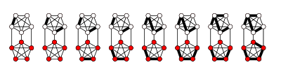
The fundamental operation of Karger’s algorithm is a form of edge contraction. The result of contracting the edge ${\displaystyle e=\{u,v\}}$ is a new node ${\displaystyle uv}$. Every edge ${\displaystyle \{w,u\}}$ or ${\displaystyle \{w,v\}}$ for ${\displaystyle w\notin \{u,v\}}$ to the endpoints of the contracted edge is replaced by an edge ${\displaystyle \{w,uv\}}$ to the new node. Finally, the contracted nodes ${\displaystyle u}$ and ${\displaystyle v}$ with all their incident edges are removed. In particular, the resulting graph contains no self-loops. The result of contracting edge ${\displaystyle e}$ is denoted ${\displaystyle G/e}$.

The contraction algorithm repeatedly contracts random edges in the graph, until only two nodes remain, at which point there is only a single cut.

The key idea of the algorithm is that it is far more likely for non min-cut edges than min-cut edges to be randomly selected and lost to contraction, since min-cut edges are usually vastly outnumbered by non min-cut edges. Subsequently, it is plausible that the min-cut edges will survive all the edge contraction, and the algorithm will correctly identify the min-cut edge.

   procedure contract(${\displaystyle G=(V,E)}$):
   while ${\displaystyle |V|>2}$
       choose ${\displaystyle e\in E}$ uniformly at random
       ${\displaystyle G\leftarrow G/e}$
   return the only cut in ${\displaystyle G}$

When the graph is represented using adjacency lists or an adjacency matrix, a single edge contraction operation can be implemented with a linear number of updates to the data structure, for a total running time of ${\displaystyle O(|V|^{2})}$. Alternatively, the procedure can be viewed as an execution of Kruskal’s algorithm for constructing the minimum spanning tree in a graph where the edges have weights ${\displaystyle w(e_{i})=\pi (i)}$ according to a random permutation ${\displaystyle \pi }$. Removing the heaviest edge of this tree results in two components that describe a cut. In this way, the contraction procedure can be implemented like Kruskal’s algorithm in time ${\displaystyle O(|E|\log |E|)}$.

The best known implementations use ${\displaystyle O(|E|)}$ time and space, or ${\displaystyle O(|E|\log |E|)}$ time and ${\displaystyle O(|V|)}$ space, respectively.^[1]

Success probability of the contraction algorithm

In a graph ${\displaystyle G=(V,E)}$ with ${\displaystyle n=|V|}$ vertices, the contraction algorithm returns a minimum cut with polynomially small probability ${\displaystyle {\binom {n}{2}}^{-1}}$. Recall that every graph has ${\displaystyle 2^{n-1}-1}$ cuts (by the discussion in the previous section), among which at most ${\displaystyle {\tbinom {n}{2}}}$ can be minimum cuts. Therefore, the success probability for this algorithm is much better than the probability for picking a cut at random, which is at most ${\displaystyle {\frac {\tbinom {n}{2}}{2^{n-1}-1}}}$.

For instance, the cycle graph on ${\displaystyle n}$ vertices has exactly ${\displaystyle {\binom {n}{2}}}$ minimum cuts, given by every choice of 2 edges. The contraction procedure finds each of these with equal probability.

To further establish the lower bound on the success probability, let ${\displaystyle C}$ denote the edges of a specific minimum cut of size ${\displaystyle k}$. The contraction algorithm returns ${\displaystyle C}$ if none of the random edges deleted by the algorithm belongs to the cutset ${\displaystyle C}$. In particular, the first edge contraction avoids ${\displaystyle C}$, which happens with probability ${\displaystyle 1-k/|E|}$. The minimum degree of ${\displaystyle G}$ is at least ${\displaystyle k}$ (otherwise a minimum degree vertex would induce a smaller cut where one of the two partitions contains only the minimum degree vertex), so ${\displaystyle |E|\geqslant nk/2}$. Thus, the probability that the contraction algorithm picks an edge from ${\displaystyle C}$ is

${\displaystyle {\frac {k}{|E|}}\leqslant {\frac {k}{nk/2}}={\frac {2}{n}}.}$

The probability ${\displaystyle p_{n}}$ that the contraction algorithm on an ${\displaystyle n}$-vertex graph avoids ${\displaystyle C}$ satisfies the recurrence ${\displaystyle p_{n}\geqslant \left(1-{\frac {2}{n}}\right)p_{n-1}}$, with ${\displaystyle p_{2}=1}$, which can be expanded as

${\displaystyle p_{n}\geqslant \prod _{i=0}^{n-3}{\Bigl (}1-{\frac {2}{n-i}}{\Bigr )}=\prod _{i=0}^{n-3}{\frac {n-i-2}{n-i}}={\frac {n-2}{n}}\cdot {\frac {n-3}{n-1}}\cdot {\frac {n-4}{n-2}}\cdots {\frac {3}{5}}\cdot {\frac {2}{4}}\cdot {\frac {1}{3}}={\binom {n}{2}}^{-1}\,.}$

Repeating the contraction algorithm

By repeating the contraction algorithm ${\displaystyle T={\binom {n}{2}}\ln n}$ times with independent random choices and returning the smallest cut, the probability of not finding a minimum cut is

${\displaystyle \left[1-{\binom {n}{2}}^{-1}\right]^{T}\leq {\frac {1}{e^{\ln n}}}={\frac {1}{n}}\,.}$

The total running time for ${\displaystyle T}$ repetitions for a graph with ${\displaystyle n}$ vertices and ${\displaystyle m}$ edges is ${\displaystyle O(Tm)=O(n^{2}m\log n)}$.

Karger–Stein algorithm

An extension of Karger’s algorithm due to David Karger and Clifford Stein achieves an order of magnitude improvement.^[3]

The basic idea is to perform the contraction procedure until the graph reaches ${\displaystyle t}$ vertices.

   procedure contract(${\displaystyle G=(V,E)}$, ${\displaystyle t}$):
   while ${\displaystyle |V|>t}$
       choose ${\displaystyle e\in E}$ uniformly at random
       ${\displaystyle G\leftarrow G/e}$
   return ${\displaystyle G}$

The probability ${\displaystyle p_{n,t}}$ that this contraction procedure avoids a specific cut ${\displaystyle C}$ in an ${\displaystyle n}$-vertex graph is

${\displaystyle p_{n,t}\geq \prod _{i=0}^{n-t-1}{\Bigl (}1-{\frac {2}{n-i}}{\Bigr )}={\binom {t}{2}}{\Bigg /}{\binom {n}{2}}\,.}$

This expression is approximately ${\displaystyle t^{2}/n^{2}}$ and becomes less than ${\displaystyle {\frac {1}{2}}}$ around ${\displaystyle t=n/{\sqrt {2}}}$. In particular, the probability that an edge from ${\displaystyle C}$ is contracted grows towards the end. This motivates the idea of switching to a slower algorithm after a certain number of contraction steps.

   procedure fastmincut(${\displaystyle G=(V,E)}$):
   if ${\displaystyle |V|\leq 6}$:
       return contract(${\displaystyle G}$, ${\displaystyle 2}$)
   else:
       ${\displaystyle t\leftarrow \lceil 1+|V|/{\sqrt {2}}\rceil }$
       ${\displaystyle G_{1}\leftarrow }$ contract(${\displaystyle G}$, ${\displaystyle t}$)
       ${\displaystyle G_{2}\leftarrow }$ contract(${\displaystyle G}$, ${\displaystyle t}$)
       return min{fastmincut(${\displaystyle G_{1}}$), fastmincut(${\displaystyle G_{2}}$)}

Analysis

The contraction parameter ${\displaystyle t}$ is chosen so that each call to contract has probability at least 1/2 of success (that is, of avoiding the contraction of an edge from a specific cutset ${\displaystyle C}$). This allows the successful part of the recursion tree to be modeled as a random binary tree generated by a critical Galton–Watson process, and to be analyzed accordingly.^[3]

The probability ${\displaystyle P(n)}$ that this random tree of successful calls contains a long-enough path to reach the base of the recursion and find ${\displaystyle C}$ is given by the recurrence relation

${\displaystyle P(n)=1-\left(1-{\frac {1}{2}}P\left({\Bigl \lceil }1+{\frac {n}{\sqrt {2}}}{\Bigr \rceil }\right)\right)^{2}}$

with solution ${\displaystyle P(n)=\Omega \left({\frac {1}{\log n}}\right)}$. The running time of fastmincut satisfies

${\displaystyle T(n)=2T\left({\Bigl \lceil }1+{\frac {n}{\sqrt {2}}}{\Bigr \rceil }\right)+O(n^{2})}$

with solution ${\displaystyle T(n)=O(n^{2}\log n)}$. To achieve error probability ${\displaystyle O(1/n)}$, the algorithm can be repeated ${\displaystyle O(\log n/P(n))}$ times, for an overall running time of ${\displaystyle T(n)\cdot {\frac {\log n}{P(n)}}=O(n^{2}\log ^{3}n)}$. This is an order of magnitude improvement over Karger’s original algorithm.^[3]

Improvement bound

To determine a min-cut, one has to touch every edge in the graph at least once, which is ${\displaystyle \Theta (n^{2})}$ time in a dense graph. The Karger–Stein's min-cut algorithm takes the running time of ${\displaystyle O(n^{2}\ln ^{O(1)}n)}$, which is very close to that.

References

- ^ a b Karger, David (1993). "Global Min-cuts in RNC and Other Ramifications of a Simple Mincut Algorithm". Proc. 4th Annual ACM-SIAM Symposium on Discrete Algorithms.
- ^ Stoer, M.; Wagner, F. (1997). "A simple min-cut algorithm". Journal of the ACM. 44 (4): 585. doi:10.1145/263867.263872. S2CID 15220291.
- ^ a b c Karger, David R.; Stein, Clifford (1996). "A new approach to the minimum cut problem" (PDF). Journal of the ACM. 43 (4): 601. doi:10.1145/234533.234534. S2CID 5385337.