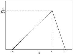
a : a ∈ ( − ∞ , ∞ ) {\displaystyle a:~a\in (-\infty ,\infty )} b : b > a {\displaystyle b:~b>a} c : a ⩽ c ⩽ b {\displaystyle c:~a\leqslant c\leqslant b}
a ⩽ x ⩽ b {\displaystyle a\leqslant x\leqslant b}
{ 2 ( x − a ) ( b − a ) ( c − a ) d l a a ⩽ x ⩽ c 2 ( b − x ) ( b − a ) ( b − c ) d l a c ⩽ x ⩽ b {\displaystyle \left\{{\begin{matrix}{\frac {2(x-a)}{(b-a)(c-a)}}&\mathrm {dla\ } a\leqslant x\leqslant c\\&\\{\frac {2(b-x)}{(b-a)(b-c)}}&\mathrm {dla\ } c\leqslant x\leqslant b\end{matrix}}\right.}
{ ( x − a ) 2 ( b − a ) ( c − a ) d l a a ⩽ x ⩽ c 1 − ( b − x ) 2 ( b − a ) ( b − c ) d l a c ⩽ x ⩽ b {\displaystyle \left\{{\begin{matrix}{\frac {(x-a)^{2}}{(b-a)(c-a)}}&\mathrm {dla\ } a\leqslant x\leqslant c\\&\\1-{\frac {(b-x)^{2}}{(b-a)(b-c)}}&\mathrm {dla\ } c\leqslant x\leqslant b\end{matrix}}\right.}
a + b + c 3 {\displaystyle {\frac {a+b+c}{3}}}
{ a + ( b − a ) ( c − a ) 2 d l a c ⩾ b − a 2 b − ( b − a ) ( b − c ) 2 d l a c ⩽ b − a 2 {\displaystyle \left\{{\begin{matrix}a+{\frac {\sqrt {(b-a)(c-a)}}{\sqrt {2}}}&\mathrm {dla\ } c\!\geqslant \!{\frac {b\!-\!a}{2}}\\&\\b-{\frac {\sqrt {(b-a)(b-c)}}{\sqrt {2}}}&\mathrm {dla\ } c\!\leqslant \!{\frac {b\!-\!a}{2}}\end{matrix}}\right.}
c {\displaystyle c}
a 2 + b 2 + c 2 − a b − a c − b c 18 {\displaystyle {\tfrac {a^{2}+b^{2}+c^{2}-ab-ac-bc}{18}}}
2 ( a + b − 2 c ) ( 2 a − b − c ) ( a − 2 b + c ) 5 ( a 2 + b 2 + c 2 − a b − a c − b c ) 3 2 {\displaystyle {\tfrac {{\sqrt {2}}(a\!+\!b\!-\!2c)(2a\!-\!b\!-\!c)(a\!-\!2b\!+\!c)}{5(a^{2}\!+\!b^{2}\!+\!c^{2}\!-\!ab\!-\!ac\!-\!bc)^{\frac {3}{2}}}}}
− 3 5 {\displaystyle -{\frac {3}{5}}}
1 2 + ln ( b − a 2 ) {\displaystyle {\frac {1}{2}}+\ln \left({\frac {b-a}{2}}\right)}
2 ( b − c ) e a t − ( b − a ) e c t + ( c − a ) e b t ( b − a ) ( c − a ) ( b − c ) t 2 {\displaystyle 2{\tfrac {(b\!-\!c)e^{at}\!-\!(b\!-\!a)e^{ct}\!+\!(c\!-\!a)e^{bt}}{(b-a)(c-a)(b-c)t^{2}}}}
− 2 ( b − c ) e i a t − ( b − a ) e i c t + ( c − a ) e i b t ( b − a ) ( c − a ) ( b − c ) t 2 {\displaystyle -2{\tfrac {(b\!-\!c)e^{iat}\!-\!(b\!-\!a)e^{ict}\!+\!(c\!-\!a)e^{ibt}}{(b-a)(c-a)(b-c)t^{2}}}}
Rozkład trójkątny – ciągły rozkład prawdopodobieństwa zmiennej losowej.
Gęstość prawdopodobieństwa rozkładu trójkątnego symetrycznego można też wyrazić jako:
gdzie: